
Visualizing Temperature Change, Extremes, and ENSO in Southeast Asia#
Project Overview
Climate change is not expressed only as a gradual increase in average temperature. Changes in temperature variability, seasonal conditions, and extreme heat can reveal different aspects of a changing climate. Natural climate variability can also temporarily amplify or offset the long-term warming signal.
In this project, you will use climate-model simulations for your assigned city in Southeast Asia to investigate four related questions:
How is temperature changing over time, and how does the seasonal cycle change?
How are extreme temperatures changing, and what do GEV distributions tell us about rare heat events?
How are historical temperatures associated with different ENSO phases?
What new climate question can you find in the data with the help of an AI agent, and how do you know your answer is right?
The project is designed to combine climate data analysis, statistical modelling, and creative visualization. You should focus on communicating the main patterns clearly rather than producing a large number of separate plots.
Submission Guide
Deadline: Tuesday 11:59 pm, 1st December 2026 (Note: Late submissions will not be accepted).
You must submit your project to Canvas. Please upload a Jupyter Notebook with the name “FinalProject_StudentID.ipynb”. You need to include your codes, figures, and the required write-ups in a single Jupyter Notebook file. Make sure to write down your student ID and full name in the cell below.
For any questions, feel free to contact Prof. Xiaogang HE (hexg@nus.edu.sg) or Yifan LU (yifan_lu@u.nus.edu).
### Fill your student ID and full name below.

# Student ID:
# Full name:
Data Description#
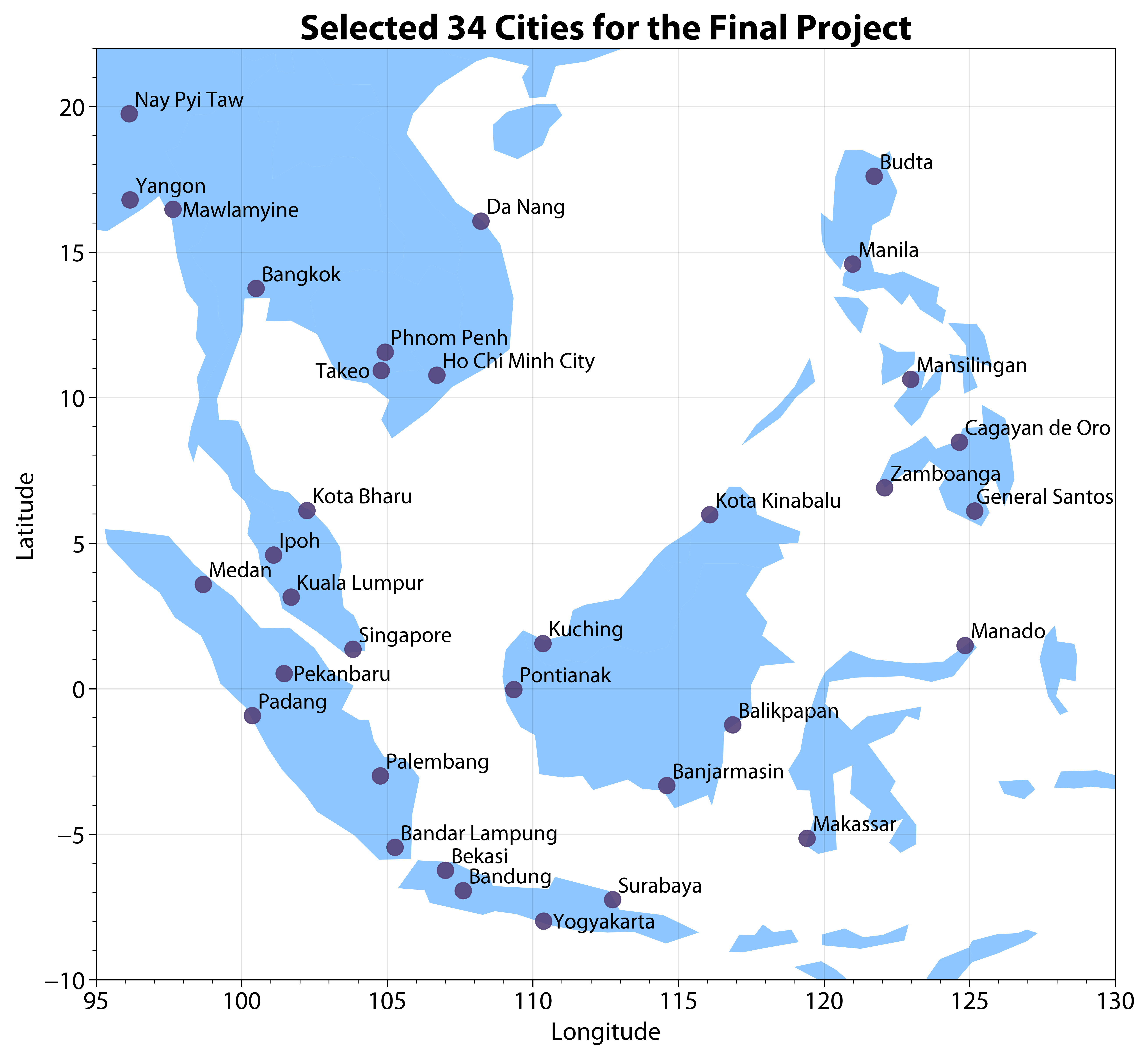
Each of you has been randomly assigned a city in Southeast Asia (see Figure below) according to your student ID. For this project, you only need to work on the city assigned to you. Simulated near-surface air temperature (tas, unit: K) from the latest climate models have been provided (available here, you can load the data directly without downloading using the example provided below). This data have been divided into two parts: historical (1850.01.01-2014.12.31) simulations (CityName_hist.csv) and future (2015.01.01-2099.12.31) projections (CityName_future.csv). Historical data contains 12 climate models and 60265 time steps. Future data contains 12 climate models and 31046 time steps in 2 climate scenarios (ssp245: middle-of-the-road scenario; ssp585: fossil-fuel based development; check SSP details here).
# Run the following script to obtain the city assigned to you.
# Note: You must use the assigned city for this project.

def getCityName(studentID):

    import json
    import urllib.request

    url = "https://raw.githubusercontent.com/XiaogangHe/python-climate-visuals/master/assets/data/2026_FinalProject_Student_City.json"
    with urllib.request.urlopen(url) as response:
        studentCity = json.load(response)

    if studentID not in studentCity.keys():
        raise ValueError('%s is not a correct student ID!'%studentID)
    else:
        return studentCity[studentID]

# Example: (please use your own ID)
studentID = 'E0000000'
cityName = getCityName(studentID)

print(cityName)
An example is provided on how to load the temperature data for historical (tas_hist) and future (tas_ssp245, tas_ssp585) simulations from the provided .csv files. For more details on data loading and preprocessing, please check the Pandas tutorial.
# Run the following script to obtain the data assigned to you.
# cityName = "Singapore"

def load_data(cityName):

    import pandas as pd
    url = "https://raw.githubusercontent.com/XiaogangHe/python-climate-visuals/master/assets/data/finalproject"
    hist_address = url + "/" + cityName + "_hist.csv"
    future_address = url + "/" + cityName + "_future.csv"
    soi_address = url + "/soi.txt"

    # Refer to https://pandas.pydata.org/pandas-docs/stable/user_guide/advanced.html
    # for more details about MultiIndex of DataFrame
    hist = pd.read_csv(hist_address, header=[0,1],
                       index_col=0, parse_dates=True)
    idx = pd.IndexSlice
    # huss_hist = hist.loc[:,idx["huss",:]].droplevel(level=0,axis=1)
    tas_hist = hist.loc[:,idx["tas",:]].droplevel(level=0,axis=1)

    future = pd.read_csv(future_address, header=[0,1,2], index_col=0, parse_dates=True)

    # huss_ssp245 = future.loc[:,idx["huss","ssp245",:]].droplevel(level=[0,1],axis=1)
    # huss_ssp585 = future.loc[:,idx["huss","ssp585",:]].droplevel(level=[0,1],axis=1)
    tas_ssp245 = future.loc[:,idx["tas","ssp245",:]].droplevel(level=[0,1],axis=1)
    tas_ssp585 = future.loc[:,idx["tas","ssp585",:]].droplevel(level=[0,1],axis=1)

    # Monthly standardized SOI (NOAA). The file is fixed-width: a 4-character
    # year followed by twelve 6-character monthly values.
    soi = pd.read_fwf(soi_address, widths=[4] + [6]*12, skiprows=4, header=None,
                      names=["year"] + list(range(1, 13)), index_col=0)
    soi = soi.stack()
    soi.index = pd.to_datetime([f"{year}-{month:02d}-01" for year, month in soi.index])
    soi.name = "soi"

    return tas_hist, tas_ssp245, tas_ssp585, soi

tas_hist, tas_ssp245, tas_ssp585, soi = load_data(cityName)
Task 1: Long-Term Temperature Changes (20 marks)#
Investigate how the temperature of your assigned city has changed from the historical period into the future.
Your analysis should reveal both the long-term warming signal and any changes in the seasonal character of temperature. Consider the historical climate in relation to the pre-industrial period, and compare future conditions under SSP2-4.5 and SSP5-8.5.
Your visualization should make it possible to assess:
how temperature has changed over time;
how much the different climate models agree or disagree;
whether warming is distributed similarly throughout the year.
Use an appropriate baseline for calculating temperature anomalies and choose a visualization or combination of visualizations that communicates these changes effectively.
Bonus: 10 marks
While you can create 24 (12 climate models × 2 climate scenarios) similar warming stripes, we hope you could come up with some creative design (e.g., layout, chart types) that are sufficiently compact to allow for meaningful comparison between periods, seasons, models, and future scenarios.
# Your solutions go here.
# Use the + icon in the toolbar to add a cell.
Task 2: Extreme Heat and Generalized Extreme Value Distributions (30 marks)#
Extreme temperatures can change differently from the average temperature. In this task, use the Generalized Extreme Value (GEV) distribution to investigate how the characteristics of rare heat events change over time.
Focus on two seasons:
June–September
December–February
Note: Some seasons span two calendar years (e.g., December–February). Pay careful attention to how you define and assign these seasons when calculating seasonal statistics, annual maxima, or comparing years.
Seasonal temperature extremes
Construct a time series of seasonal maximum temperatures for each year for the following periods:
1850–1900 — pre-industrial baseline;
1950–2014 — historical period;
2015–2099 — SSP2-4.5;
2015–2099 — SSP5-8.5.
For this task, use the multi-model mean temperature series.
GEV analysis
To do this:
Fit a Generalized Extreme Value (GEV) distribution using Maximum Likelihood Estimation (MLE) to the seasonal maxima for each period, season, and future scenario.
Assess the quality of your fitted distributions.
Visualize the shift in your fitted GEV distributions over different periods and scenarios. (Hint: You may use visualization tools such as Ridgeline plot)
Using the fitted GEV distributions to estimate the 1-in-100-year and 1-in-1000-year return level. Then, compare how these values change between periods and scenarios.
# Your solutions go here.
# Use the + icon in the toolbar to add a cell.
Task 3: Temperature and ENSO Variability (15 marks)#
Long-term warming occurs alongside substantial year-to-year climate variability. In this task, investigate whether historical temperature conditions differ between El Niño and La Niña years using the Southern Oscillation Index (SOI).
This analysis is restricted to 1951–2014, for which the accompanying monthly SOI record is available. The project materials include monthly standardized SOI values. Use these values to derive a single SOI-based ENSO classification for each year, based on the calendar-year (January–December) mean of the monthly SOI:
Positive annual mean SOI → La Niña
Negative annual mean SOI → El Niño
For this task, focus specifically on June–September. Investigate whether temperature conditions during this season differ between the two SOI-based ENSO phases.
Your analysis should consider both typical temperature conditions and extreme heat. Use appropriate visualizations to compare the temperature distributions and investigate whether unusually warm June–September seasons occur with different frequencies between El Niño and La Niña years.
Bonus (10 marks)
Before comparing El Niño and La Niña years, here’s something to think about: Long-term warming. El Niño and La Niña years may not be spread evenly across 1951–2014. If one phase occurs more often in later, warmer decades, it can look warmer even without any real ENSO effect. Remove the long-term trend from your June–September temperatures (e.g., subtract a linear trend) before comparing the two phases, and check how your results change with and without detrending.
# Your solutions go here.
# Use the + icon in the toolbar to add a cell.
Task 4: Agent-Assisted Exploration (20 marks)#
In Tasks 1–3, the questions were given to you. In this task, you find one yourself. Use an AI coding/analysis agent (e.g., ChatGPT, Claude, Gemini, GitHub Copilot) as a research partner for the whole process (finding a question → analysing it → checking the result), not only as a code writer.
Starting from your ENSO analysis in Task 3, work with the agent to identify and investigate one new climate question about your assigned city. The question should go beyond what Tasks 1–3 already ask. It may extend one of them or come from something you notice in the data. Possible directions:
warming trends
extreme temperatures
model uncertainty
year-to-year variability
an unusual pattern you discover in the data
Your Task 4 should include:
Question and motivation — what you asked, why it is interesting, and how you arrived at it with the agent.
Analysis — code and one or two figures that answer the question.
Validation — evidence that your result reflects the climate data, not a mistake in the code or in the data handling.
Answer — a short interpretation, including the limitations of your analysis.
Rules:
Use only the data provided for this project (the temperature simulations and the SOI record).
Parts 1, 3 and 4 are written content and must be in your own words (see AI policies).
Marking: question and analysis (10), validation and interpretation (5), Agent Use Log (5).
# Your solutions go here.
# Use the + icon in the toolbar to add a cell.
Agent Use Log#
Agent(s) used: (tool and model, e.g., “Claude, Sonnet”)
Key prompts (2–3): (what are some of the main guidance you provided)
One useful suggestion: (what the agent suggested, and how you used it)
One rejected or corrected suggestion: (what the agent suggested, why it was wrong or unsuitable, how you found out, and what you did instead)
Sanity checks 1 & 2: (what you checked, how you checked it, and the result)
A sanity check compares a result against something you know independently — for example, a value calculated by hand for one year, the units, or a plot of the raw series. “The code ran without errors” is not a sanity check.
# Your write-ups go here.
# Use the + icon in the toolbar to add a cell.
Short Write-ups (15 marks)#
What story are you trying to tell? (Hints: You could discuss major findings from your analysis, key takeaways, and possible implications.)
Why did you choose such a visual design and how does it facilitate effective communication? (Hint: you could provide some rationale in terms of your choice of chart types, use of color, size, etc.)
# Your write-ups go here.
# Use the + icon in the toolbar to add a cell.
Reminder
The goal is to communicate more information without simply adding more separate plots. Feel free to make your own design. You can utilize ChatGPT for better data storytelling, such as creating dashboards or animation.
Final Words#
You may recycle your code from HW1 and HW2 where appropriate.
Remember to:
check your date and seasonal selections carefully, especially when working with seasons that span two calendar years;
make your figures readable and understandable without requiring the reader to inspect the code;
consider the principles in the official IPCC Visual Style Guide when designing your figures.
For this final project, quality matters more than quantity. A small number of thoughtful, well-designed figures is much more valuable than a large collection of repetitive plots.
Enjoy coding!
AI policies#
You can use ChatGPT (or other AI tools) for coding, visualization design, and related tasks, and Task 4 requires you to use an AI agent. However, AI should not be used for any written content: the short write-ups, the written parts of Task 4 (question and motivation, validation, answer), and the descriptions in your Agent Use Log must be your own.
For AI use outside Task 4, add a one-line acknowledgement at the end of your notebook (tool, date, and what it was used for).
Reference#
National Centers for Environmental Information. (2026). El Niño / Southern Oscillation (ENSO). https://www.ncei.noaa.gov/access/monitoring/enso/soi#calculation-of-soi