
2.1. NumPy tutorial#
NumPy is the core package for scientific computing in Python. It vastly simplifies manipulating and crunching vectors and matrices. Many of other leading packages rely on NumPy as a infrastructure piece.
In this tutorial, we will cover:
numpy: Array, Array Indexing, Array Manipulation, Array Math & Broadcasting.
To use NumPy, we need to import the numpy package at first:
import numpy as np
print(np.__version__)
1.21.5
2.1.1. Array and its Creation#
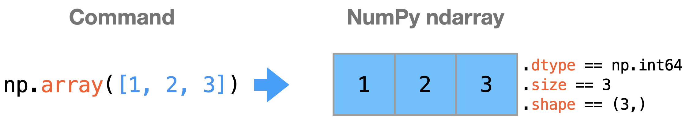
A NumPy array (a.k.a. ndarray) is the core of this package. ndarray is a grid of values, all of the same type – quite like a special version of list. We can create a NumPy array by passing a python list to it using np.array(). NumPy will try to guess a datatype if we do not set it explicitly. Within the ndarray object, some properties are provided for us to know the status of it, such as dtype – datatype of elements, size – number of elements, shape – sizes of all dimensions, etc.
a = np.array([1, 2, 3])  # Create a rank 1 array from a list
print(a, type(a))
print(a.shape, a.dtype, a[0])
[1 2 3] <class 'numpy.ndarray'>
(3,) int64 1
Using a list of lists with the same size, we could create 2D, 3D, or even higher dimensional arrays.
b = np.array([[1, 2, 3, 4], [5, 6, 7, 8]])  # Create a rank 2 array
print(b, b.shape, b[1, 2])

c = np.array([[[111, 112, 113, 114], [121, 122, 123, 124]],
              [[211, 212, 213, 214], [221, 222, 223, 224]],
              [[311, 312, 313, 314], [321, 322, 323, 324]]])
                                            # Create a rank 3 array
print(c, c.shape, c[0, 1, 2])
[[1 2 3 4]
 [5 6 7 8]] (2, 4) 7
[[[111 112 113 114]
  [121 122 123 124]]

 [[211 212 213 214]
  [221 222 223 224]]

 [[311 312 313 314]
  [321 322 323 324]]] (3, 2, 4) 123
Numpy also provides many useful methods to create arrays for specific purposes. It’s common that some methods use a tuple to specify the shape of array you want.
d = np.arange(5, 50, 10)  # Create an array starting at 5, ending at 50, with a step of 10
d = np.zeros((2, 2))      # Create an array of all zeros with shape (2, 2)
d = np.ones((1, 2))       # Create an array of all ones with shape (1, 2)
d = np.random.random((3, 1))  # Create an array of random values with shape (3, 1)
# Try printing them
print(d)
[[0.67742525]
 [0.0784592 ]
 [0.6098676 ]]
2.1.2. Array Indexing#
The most common ways to pull out a section of arrays include slicing, integer array indexing and Boolean array indexing. We may choose the appropriate indexing methods for different purposes.
Slicing
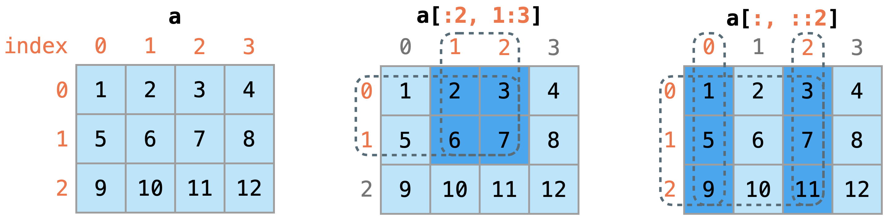
We could specify an index slice in the form start:end or start:end:step for each dimension of the array to access subarrays, quite similar to slicing python list.
a = np.array([[1, 2, 3, 4], [5, 6, 7, 8], [9, 10, 11, 12]])
print(a[:2, 1:3])  # Slice 1st to 2nd rows and 2nd to 3rd columns
print(a[:, ::2])   # Slice all odd columns
[[2 3]
 [6 7]]
[[ 1  3]
 [ 5  7]
 [ 9 11]]
Note that a slice of an array is always a view of the same data, so modifying it will modify the original array. If you wish to avoid this, you could use the copy() method to create a soft copy when assigned to a new variable. This is also true when you assign the whole array to another variable.
a = np.array([[1, 2, 3, 4], [5, 6, 7, 8], [9, 10, 11, 12]])
b1 = a[:2, 1:3]
b1[0, 0] = 77    # b[0, 0] will be the same piece of data as a[0, 1]
print(b1[0, 0], a[0, 1])

a = np.array([[1, 2, 3, 4], [5, 6, 7, 8], [9, 10, 11, 12]])
b2 = a[:2, 1:3].copy()
b2[0, 0] = 77
print(b2[0, 0], a[0, 1])
77 77
77 2
Integer array indexing
Integer indexing allows you to index arbitrary elements in the array by separately assign the indexing for each dimension. Note that the resulting array in this way is a copy, so modifying it will not modify the original.
a = np.array([[1, 2, 3], [4, 5, 6], [7, 8, 9], [10, 11, 12]])
print(a[[0, 1, 2], [0, 1, 0]]) # Integer indexing

# The above example of integer array indexing is equivalent to this:
print(np.array([a[0, 0], a[1, 1], a[2, 0]]))
[1 5 7]
[1 5 7]
This method is useful when we want to conduct an operation on a series of specific elements in the array.
row = [0, 1, 2]  # Explicitly express row indices
col = [0, 1, 0]  # and col indices
a[row, col] += 1000  # Only operate on specific elements
print(a)
[[1001    2    3]
 [   4 1005    6]
 [1007    8    9]
 [  10   11   12]]
You can also mix integer indexing with slice indexing to obtain a subarray. However, note that mixing yields an array of lower rank, while using only slices yields an array of the same rank as the original array.
a = np.array([[1, 2, 3], [4, 5, 6], [7, 8, 9], [10, 11, 12]])
a_1row = a[0, :]     # Mix integer indexing with slice indexing
a_2rows = a[0:1, :]  # Slice indexing
print(a_1row, a_1row.shape)   # Lower rank
print(a_2rows, a_2rows.shape)
[1 2 3] (3,)
[[1 2 3]] (1, 3)
Boolean array indexing
Boolean array indexing lets you pick out elements of an array based on the Boolean array with the same shape as the original one.
a = np.array([[1, 2, 3], [4, 5, 6], [7, 8, 9], [10, 11, 12]])
bool_idx = (a > 8)  # Find the elements of a that are bigger than 2;
                    # this returns a numpy array of Booleans of the same
                    # shape as a, where each slot of bool_idx tells
                    # whether that element of a is > 2.

print(bool_idx)
print(a[bool_idx])  # Boolean array indexing, return rank 1 array for True positions
[[False False False]
 [False False False]
 [False False  True]
 [ True  True  True]]
[ 9 10 11 12]
We can do all of the above in a single concise statement, which is more readable.
a[a > 8]
array([ 9, 10, 11, 12])
If you want to know more fancy indexing methods you should read the documentation.
2.1.3. Array Manipulation#
After the creation of an array, it is possible to reshape its sizes with the reshape() method.
a = np.arange(12)
print(a)
print(a.reshape((3, 4)))
print(np.reshape(a, (3, 4)))  # use the class method and put object as 1st argument is the same
[ 0  1  2  3  4  5  6  7  8  9 10 11]
[[ 0  1  2  3]
 [ 4  5  6  7]
 [ 8  9 10 11]]
[[ 0  1  2  3]
 [ 4  5  6  7]
 [ 8  9 10 11]]
To transpose an array, simply use the T property of an array object, or use the transpose() method.
a = np.arange(12).reshape((3, 4))
print("transpose through property\n", a.T)          # property is like a variable
print("transpose through method\n", a.transpose())  # method is like a function
transpose through property
 [[ 0  4  8]
 [ 1  5  9]
 [ 2  6 10]
 [ 3  7 11]]
transpose through method
 [[ 0  4  8]
 [ 1  5  9]
 [ 2  6 10]
 [ 3  7 11]]
Numpy also offers several method to join multiple arrays, such as hstack() – horizontally concatenate arrays, vstack() – vertically concatenate arrays, concatenate() – concatenate arrays across the specified axis, etc. Please mind that the shapes of input arrays must be compatible for specific joining methods.
a = np.arange(12).reshape((3, 4))
b = np.arange(8).reshape((2, 4))
c = np.arange(6).reshape((3, 2))

ac = np.hstack((a, c))
ab = np.vstack((a, b))
print(ac)
print(ab)
[[ 0  1  2  3  0  1]
 [ 4  5  6  7  2  3]
 [ 8  9 10 11  4  5]]
[[ 0  1  2  3]
 [ 4  5  6  7]
 [ 8  9 10 11]
 [ 0  1  2  3]
 [ 4  5  6  7]]
Besides reshaping and joining, arrays can also be split, tiled, and rearranged in other ways. Please refer to official documention of array manipulation when you need them.
2.1.4. Array Math#
The real power of NumPy is that arrays can be operated for mathematical calculations easily, along with a bunch of mathematical methods provided. Let’s see some examples.
2.1.4.1. Basic Arithmetic#
x = np.array([[1, 2], [3, 4]], dtype=np.float64) # Set data types of elements by dtype
y = np.array([[5, 6], [7, 8]], dtype=np.float64)

# Elementwise sum; both produce an array
print(x + y)
print(np.add(x, y))
[[ 6.  8.]
 [10. 12.]]
[[ 6.  8.]
 [10. 12.]]
# Elementwise square root; produces an array
print(np.sqrt(x))
# Elementwise natural logarithm; produces an array
print(np.log(x))
[[1.         1.41421356]
 [1.73205081 2.        ]]
[[0.         0.69314718]
 [1.09861229 1.38629436]]
NumPy also supports matrix multiplication. We use dot() function to compute inner products of vectors, to multiply a vector by a matrix, and to multiply matrices.
x = np.array([[1, 2], [3, 4]])
y = np.array([[5, 6], [7, 8]])

# Inner product of vectors
print(x[0, :].dot(y[0, :]))
print(np.dot(x[0, :], y[0, :]))
# Matrix / matrix product
print(x.dot(y))
print(np.dot(x, y))
17
17
[[19 22]
 [43 50]]
[[19 22]
 [43 50]]
2.1.4.2. Aggregation Calculations#
Additional benefits NumPy gives us are aggregation functions, with which we could get basic statistics of array along different axes. These include min()/max() – get minimum/maximum value, sum() – summation, mean() – average, std() - standard deviation, and plenty of others.
x = np.array([[1, 2, 3], [4, 5, 6]])

print(np.sum(x))          # Sum of all elements; produce a value
print(np.sum(x, axis=0))  # Sum along axis 0 (column); produce a lower rank array
print(x.sum(axis=1))      # Sum along axis 1 (row); produce a lower rank array
# Try others!
21
[5 7 9]
[ 6 15]
As you may observe above, we could specify which axis to perform aggregation calculations, but sometimes we may get confused on which one to use so we get what we want, especially when it comes to higher dimensions. Hope the following figure and code help you to comprehend the axis number.
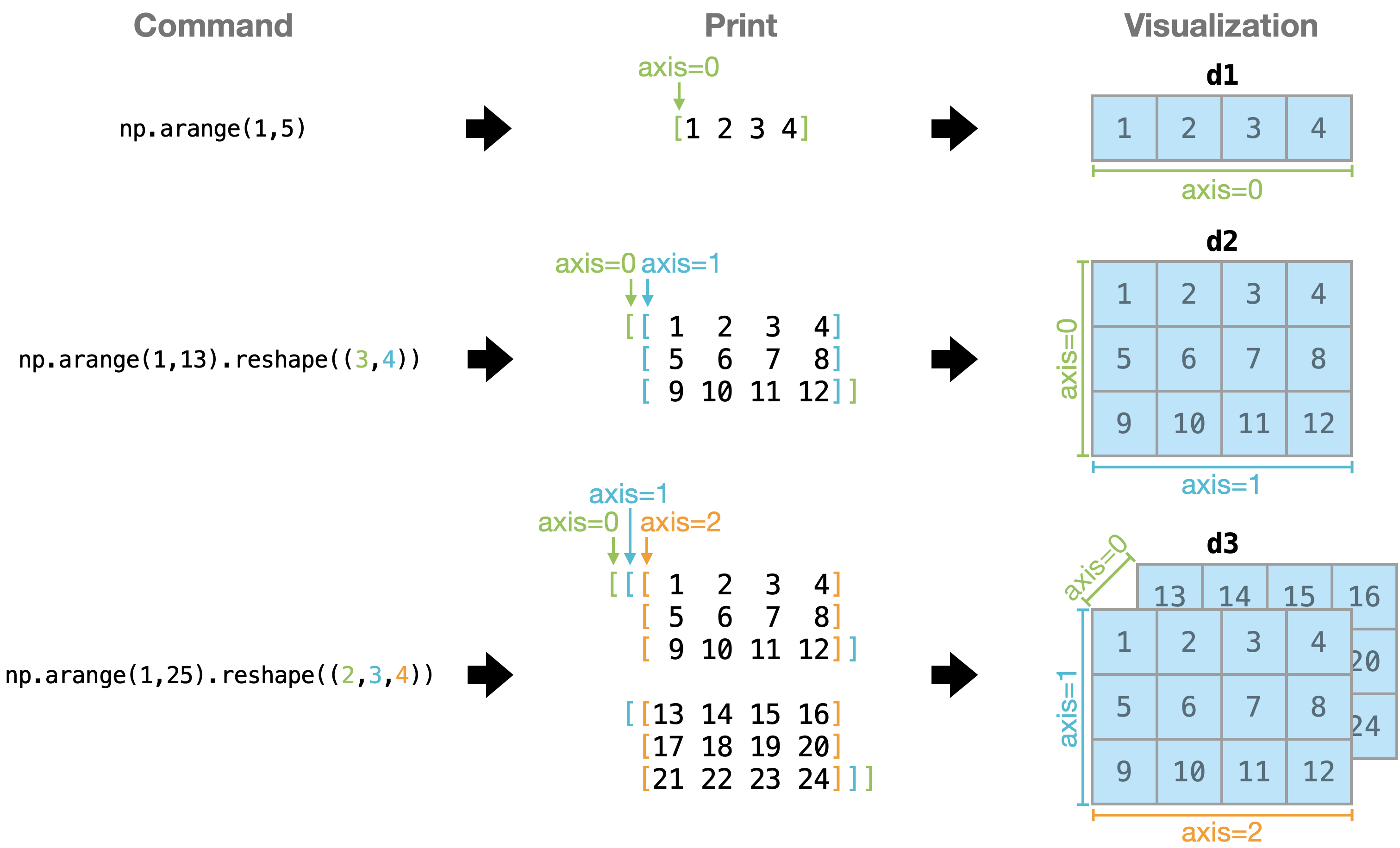
d1 = np.arange(1, 5)
d2 = np.arange(1, 13).reshape((3, 4))
d3 = np.arange(1, 25).reshape((2, 3, 4))

print("Minimum along axis 0:")
print(d3.min(axis=0))  # ❓: Why we have this result?
Minimum along axis 0:
[[ 1  2  3  4]
 [ 5  6  7  8]
 [ 9 10 11 12]]
2.1.5. One more thing: Broadcasting#
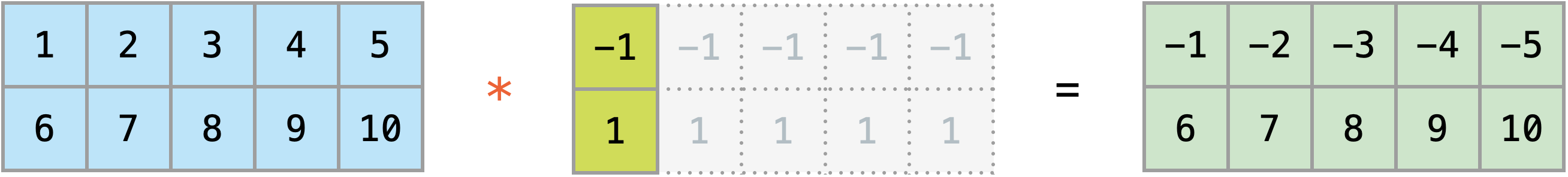
Broadcasting is another powerful NumPy mechanism that allows arrays of different shapes to work together when performing arithmetic operations. Let’s see an example of dividing an array by a scalar, and an example of changing signs by rows through multiplying.
x = np.arange(1, 11).reshape((2, 5))
x_norm = x / 10
print(x_norm)

sign = np.array([-1, 1]).reshape((2, 1))
x_signed = x * sign
print(x_signed)
[[0.1 0.2 0.3 0.4 0.5]
 [0.6 0.7 0.8 0.9 1. ]]
[[-1 -2 -3 -4 -5]
 [ 6  7  8  9 10]]
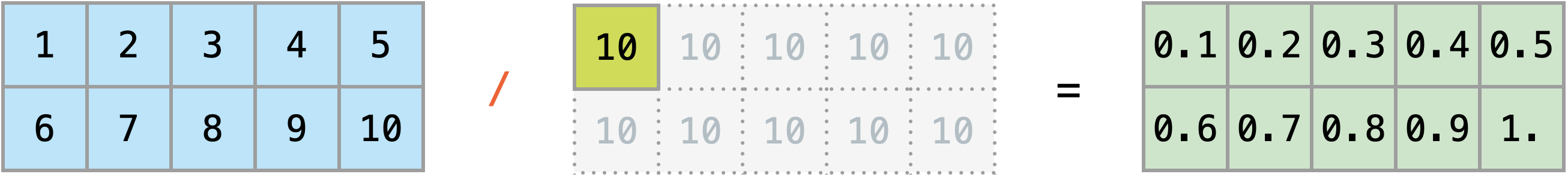
We could see that when shapes of both arrays are compatible, NumPy would automatically stretch (replicating) arrays as above so that arithmetic calculations can be directly applied. But how can we know array shapes are compatible? 🤔
NumPy compares array shapes from back forward. It starts with the trailing (i.e. rightmost) dimensions and works its way left. For each dimension of both arrays, their sizes are compatible when
they are equal, or
one of them is 1
If these conditions are not met, a ValueError: operands could not be broadcast together exception will be thrown, indicating array shapes incompatible. Maybe some compatible examples are more straightforward for us to get a sense of this rule. Let’s say we operate between A and B having the following shapes.
A      (2d array):  5 x 4
B      (1d array):      1
Result (2d array):  5 x 4

A      (2d array):  5 x 4
B      (1d array):      4
Result (2d array):  5 x 4

A      (3d array):  15 x 3 x 5 # also work for higher dimensions
B      (3d array):  15 x 1 x 5
Result (3d array):  15 x 3 x 5

A      (3d array):  15 x 1 x 5
B      (2d array):       3 x 1
Result (3d array):  15 x 3 x 5
Numpy will automatically broadcast the dimensions that are different between A and B. Here are examples not compatible.
A      (1d array):  3
B      (1d array):  4 # trailing dimension not match ❌

A      (2d array):      2 x 1
B      (3d array):  8 x 4 x 3 # second from last dimensions mismatch ❌
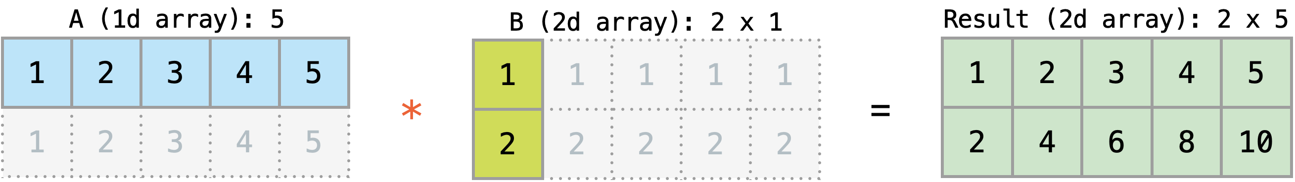
One successful and interesting broadcasting example is to calculate outer product of two vectors.
A = np.arange(1, 6)
B = np.arange(1, 3).reshape((2, 1))  # ❓: why we need reshape?

Result = A * B
print(Result)
[[ 1  2  3  4  5]
 [ 2  4  6  8 10]]
Broadcasting typically makes your code more concise, readable, and more importantly, faster.
2.1.6. References#
This tutorial was edited based on the Python Numpy Tutorial, and referred to Jay Alammar’s Visual Intro to NumPy.
This tutorial has touched on many important things you need about
numpy, but is far from complete. Check out more on numpy documentation.If you are already familiar with MATLAB, you might find this tutorial useful to help distinguish between
numpyand MATLAB.