Visualizing Climate Change’s Impact on Water Demand for Crop in Southeast Asia under Extreme Heat#
Project Overview
Design creative visualizations to unravel the impact of extreme heat and the associated crop water demand in Southeast Asia using the latest climate model simulations.
Submission Guide
Deadline: Tuesday 11:59 pm, 2nd December 2025 (Note: Late submissions will not be accepted).
You must submit your project to Canvas. Please upload a Jupyter Notebook with the name “FinalProject_StudentID.ipynb”. You need to include your codes, figures, and the required write-ups in a single Jupyter Notebook file. Make sure to write down your student ID and full name in the cell below.
For any questions, feel free to contact Prof. Xiaogang HE (hexg@nus.edu.sg), Yifan LU (yifan_lu@u.nus.edu), or Kewei ZHANG (kewei_zhang@u.nus.edu).
### Fill your student ID and full name below.

# Student ID:
# Full name:
Data Description#
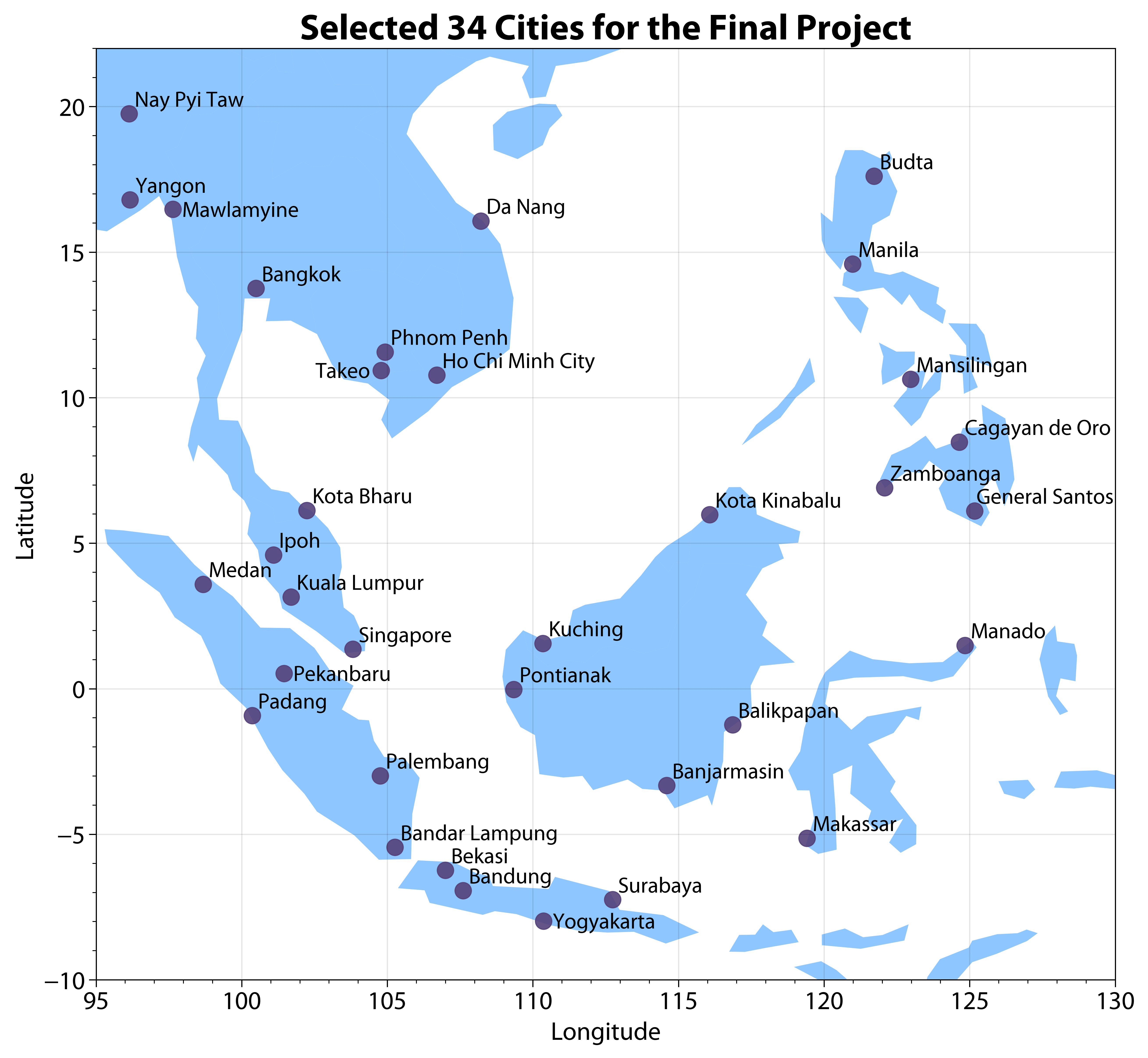
Each of you has been randomly assigned a city in Southeast Asia (see Figure below) according to your student ID. For this project, you only need to work on the city assigned to you. Simulated near-surface air temperature (tas, unit: K) from the latest climate models have been provided (available here, you can load the data directly without downloading using the example provided below). This data have been divided into two parts: historical (1850.01.01-2014.12.31) simulations (CityName_hist.csv) and future (2015.01.01-2099.12.31) projections (CityName_future.csv). Historical data contains 12 climate models and 60265 time steps. Future data contains 12 climate models and 31046 time steps in 2 climate scenarios (ssp245: sustainable development scenario; ssp585: fossil-fuel based development; check SSP details here).
# Run the following script to obtain the city assigned to you.
# Note: You must use the assigned city for this project.

def getCityName(studentID):

    import json
    import urllib.request

    url = "https://raw.githubusercontent.com/XiaogangHe/python-climate-visuals/master/assets/data/2025_FinalProject_Student_City.json"
    with urllib.request.urlopen(url) as response:
        studentCity = json.load(response)

    if studentID not in studentCity.keys():
        raise ValueError('%s is not a correct student ID!'%studentID)
    else:
        return studentCity[studentID]

# Example: (please use your own ID)
studentID = 'E0000000'
cityName = getCityName(studentID)

print(cityName)
An example is provided on how to load the temperature data for historical (tas_hist) and future (tas_ssp245, tas_ssp585) simulations from the provided .csv files. For more details on data loading and preprocessing, please check the Pandas tutorial.
# Run the following script to obtain the data assigned to you.
# cityName = "Singapore"

def load_data(cityName):

    import pandas as pd
    url = "https://raw.githubusercontent.com/XiaogangHe/python-climate-visuals/master/assets/data/finalproject"
    hist_address = url + "/" + cityName + "_hist.csv"
    future_address = url + "/" + cityName + "_future.csv"

    # Refer to https://pandas.pydata.org/pandas-docs/stable/user_guide/advanced.html
    # for more details about MultiIndex of DataFrame
    hist = pd.read_csv(hist_address, header=[0,1],
                       index_col=0, parse_dates=True)
    idx = pd.IndexSlice
    # huss_hist = hist.loc[:,idx["huss",:]].droplevel(level=0,axis=1)
    tas_hist = hist.loc[:,idx["tas",:]].droplevel(level=0,axis=1)

    future = pd.read_csv(future_address, header=[0,1,2], index_col=0, parse_dates=True)

    # huss_ssp245 = future.loc[:,idx["huss","ssp245",:]].droplevel(level=[0,1],axis=1)
    # huss_ssp585 = future.loc[:,idx["huss","ssp585",:]].droplevel(level=[0,1],axis=1)
    tas_ssp245 = future.loc[:,idx["tas","ssp245",:]].droplevel(level=[0,1],axis=1)
    tas_ssp585 = future.loc[:,idx["tas","ssp585",:]].droplevel(level=[0,1],axis=1)

    return tas_hist, tas_ssp245, tas_ssp585

tas_hist, tas_ssp245, tas_ssp585 = load_data(cityName)
Task 1 (20 marks)#
Create “warming” stripes to visualize historical (1950-2014) and future (2015-2099) warming trends. You can use the annual average temperature from 1850 to 1900 as the baseline to calculate annual temperature anomalies for the required periods (1950-2014 and 2015-2099).
Bonus: 10 marks
While you can create 24 (12 climate models × 2 climate scenarios) similar warming stripes for Task 1, we hope you could come up with some creative design (e.g., layout, chart types) to visualize all information with a minimum number of graphs.
# Your solutions go here.
# Use the + icon in the toolbar to add a cell.
Task 2 (40 marks)#
Visualize the changing risks of heat extremes of different monsoon seasons based on the average simulations from multiple climate models. To do this, you need to:
Fit Generalized Extreme Value (GEV) distributions using the Maximum Likelihood Estimation (MLE) method on the seasonal maximum daily temperature during the summer monsoon (June–September) and winter monsoon (December–February) periods over different time intervals — 1850–1900 (pre-industrial baseline), 1950–2014 (historical), and 2015–2099 (future scenarios). Perform the analysis separately for different emission pathways (SSP2-4.5 and SSP5-8.5). Demonstrate and evaluate the performance of your fitted GEV distributions for each season and scenario.
Visualize the shift in your fitted GEV distributions over different periods and scenarios. (Hint: You may use visualization tools such as Ridgeline plot)
Estimate and compare the return levels for the 1-in-100-year and 1-in-1000-year heat extreme events over different periods and scenarios. Annotate the return levels in the fitted distributions.
# Your solutions go here.
# Use the + icon in the toolbar to add a cell.
Task 3 (20 marks)#
Estimating plant evapotranspiration is crucial in Southeast Asia, a major producer and exporter of crops, to determine water demand for agriculture. Accurate estimates ensure efficient irrigation, successful harvests, and food security under population growth and climate change.
Using the daily air temperature time series for your assigned city, analyze the changing crop water demand by completing the following steps:
Step 1: Calculate the total reference crop evapotranspiration (\(\mathrm{ET}_0\)) in each month based on the Blaney–Criddle Method:
\[ \mathrm{ET}_{0}=P \left(0.46 T_{\mathrm{mean}}+8\right) D \tag{1} \]where
\(\mathrm{ET}_{0}\) — Reference crop evapotranspiration \(\mathrm{[mm/month]}\)
\(P\) — Mean daily percentage of annual daytime hours (see Table 1 in the Appendix) \(\mathrm{[-]}\)
\(T_{\mathrm{mean}}\) — Mean monthly temperature \([\mathrm{^\circ C}]\)
\(D\) — Number of days in the corresponding month \(\mathrm{[day]}\)Visualize and compare the distributions of \(\mathrm{ET}_0\) across different months, for the historical period (1950-2014) and future emission scenarios (2015-2099, SSP2-4.5 and SSP5-8.5).
Step 2: Assume there is an experimental field (1 ha) in your study area planted with grain maize. Estimate the accumulated crop water demand over the planting season (October to February) using Equation (2):
\[ \mathrm{DEMAND}=\sum_{m\in M}\zeta K_c\mathrm{ET}_0 \mathrm{A} \tag{2} \]where
\(\mathrm{DEMAND}\) — Crop water demand \(\mathrm{[m^3]}\)
\(\zeta\) — Unit conversion factor \(\mathrm{[-]}\)
\(K_c\) — Crop coefficient (month-dependent, see Table 2 in the Appendix) \(\mathrm{[-]}\)
\(\mathrm{A}\) — Planting area \(\mathrm{[m^2]}\)Visualize the time series of annual water demand for the different periods and scenarios as well.
Step 3: Estimate the crop water demand during the 1-in-100-year and 1-in-1000-year heat extreme events identified in Task 2. Compare these with the historical mean daily crop water demand and discuss how much extreme events are projected to increase water consumption.
# Your solutions go here.
# Use the + icon in the toolbar to add a cell.
Short Write-ups (20 marks)#
What story are you trying to tell? (Hints: You could discuss major findings from your analysis, key takeaways, and possible implications.)
Why did you choose such a visual design and how does it facilitate effective communication? (Hint: you could provide some rationale in terms of your choice of chart types, use of color, size, etc.)
# Your write-ups go here.
# Use the + icon in the toolbar to add a cell.
Bonus: 20 marks
For both Task 1 and Task 3, design your visualizations to incorporate uncertainties from (1) climate models (which exist over the entire period from 1950-2099) and (2) climate scenarios (which only exist during 2015-2099).
Feel free to make your own design. You can utilize ChatGPT for better data storytelling, such as creating dashboards or animation.
Tips#
You can recycle your codes from HW1 and HW2.
Note the unit conversion of \(\mathrm{ET}_{0}\) and \(\mathrm{area}\) in Task 3 Step 2.
The planting season spans across two calendar years. Therefore, for the historical period from 1950 to 2014, this results in 64 complete planting seasons. The future scenario is treated analogously.
Further information on the Blaney–Criddle method is available in the FAO guidelines (Brouwer & Heibloem, 1986).
Official IPCC visual style guide can be found here.
AI policies#
You can use ChatGPT (or other AI tools) for coding, visualization design, and related tasks. However, AI should not be used for your short write-ups. All written content must be your own. If you use AI for coding or visualizations, proper citations must be provided where applicable.
Appendix#
Table 1. Reference value of \(P\) at 15°N from FAO
Month |
Jan |
Feb |
Mar |
Apr |
May |
Jun |
Jul |
Aug |
Sep |
Oct |
Nov |
Dec |
|---|---|---|---|---|---|---|---|---|---|---|---|---|
\(P\) |
0.26 |
0.26 |
0.27 |
0.28 |
0.29 |
0.29 |
0.29 |
0.28 |
0.28 |
0.27 |
0.26 |
0.25 |
Table 2. Estimated \(K_c\) for grain maize
Month |
Jan |
Feb |
Mar |
Apr |
May |
Jun |
Jul |
Aug |
Sep |
Oct |
Nov |
Dec |
|---|---|---|---|---|---|---|---|---|---|---|---|---|
\(K_c\) |
1.15 |
0.70 |
– |
– |
– |
– |
– |
– |
– |
0.40 |
0.80 |
1.15 |
Reference#
Brouwer, C., & Heibloem, M. (1986). Irrigation Water Management: Training Manual No. 3. Part II: Determination of Irrigation Water Needs.
Food and Agriculture Organization of the United Nations (FAO), Rome.
Available at: https://www.fao.org/4/s2022e/s2022e00.htm#Contents (accessed September 2025).